4 Relationships between words: n-grams and correlations
So far we’ve considered words as individual units, and considered their relationships to sentiments or to documents. However, many interesting text analyses are based on the relationships between words, whether examining which words tend to follow others immediately, or that tend to co-occur within the same documents.
In this chapter, we’ll explore some of the methods tidytext offers for calculating and visualizing relationships between words in your text dataset. This includes the token = "ngrams" argument, which tokenizes by pairs of adjacent words rather than by individual ones. We’ll also introduce two new packages: ggraph, which extends ggplot2 to construct network plots, and widyr, which calculates pairwise correlations and distances within a tidy data frame. Together these expand our toolbox for exploring text within the tidy data framework.
4.1 Tokenizing by n-gram
We’ve been using the unnest_tokens function to tokenize by word, or sometimes by sentence, which is useful for the kinds of sentiment and frequency analyses we’ve been doing so far. But we can also use the function to tokenize into consecutive sequences of words, called n-grams. By seeing how often word X is followed by word Y, we can then build a model of the relationships between them.
We do this by adding the token = "ngrams" option to unnest_tokens(), and setting n to the number of words we wish to capture in each n-gram. When we set n to 2, we are examining pairs of two consecutive words, often called “bigrams”:
library(dplyr)
library(tidytext)
library(janeaustenr)

austen_bigrams <- austen_books() %>%
  unnest_tokens(bigram, text, token = "ngrams", n = 2)

austen_bigrams
## # A tibble: 725,048 × 2
## book bigram
## <fctr> <chr>
## 1 Sense & Sensibility sense and
## 2 Sense & Sensibility and sensibility
## 3 Sense & Sensibility sensibility by
## 4 Sense & Sensibility by jane
## 5 Sense & Sensibility jane austen
## 6 Sense & Sensibility austen 1811
## 7 Sense & Sensibility 1811 chapter
## 8 Sense & Sensibility chapter 1
## 9 Sense & Sensibility 1 the
## 10 Sense & Sensibility the family
## # ... with 725,038 more rowsThis data structure is still a variation of the tidy text format. It is structured as one-token-per-row (with extra metadata, such as book, still preserved), but each token now represents a bigram.
Notice that these bigrams overlap: “sense and” is one token, while “and sensibility” is another.
4.1.1 Counting and filtering n-grams
Our usual tidy tools apply equally well to n-gram analysis. We can examine the most common bigrams using dplyr’s count():
austen_bigrams %>%
  count(bigram, sort = TRUE)
## # A tibble: 211,237 × 2
## bigram n
## <chr> <int>
## 1 of the 3017
## 2 to be 2787
## 3 in the 2368
## 4 it was 1781
## 5 i am 1545
## 6 she had 1472
## 7 of her 1445
## 8 to the 1387
## 9 she was 1377
## 10 had been 1299
## # ... with 211,227 more rowsAs one might expect, a lot of the most common bigrams are pairs of common (uninteresting) words, such as of the and to be: what we call “stop-words” (see Chapter 1). This is a useful time to use tidyr’s separate(), which splits a column into multiple based on a delimiter. This lets us separate it into two columns, “word1” and “word2”, at which point we can remove cases where either is a stop-word.
library(tidyr)

bigrams_separated <- austen_bigrams %>%
  separate(bigram, c("word1", "word2"), sep = " ")

bigrams_filtered <- bigrams_separated %>%
  filter(!word1 %in% stop_words$word) %>%
  filter(!word2 %in% stop_words$word)

# new bigram counts:
bigram_counts <- bigrams_filtered %>%
  count(word1, word2, sort = TRUE)

bigram_counts
## Source: local data frame [33,421 x 3]
## Groups: word1 [6,711]
##
## word1 word2 n
## <chr> <chr> <int>
## 1 sir thomas 287
## 2 miss crawford 215
## 3 captain wentworth 170
## 4 miss woodhouse 162
## 5 frank churchill 132
## 6 lady russell 118
## 7 lady bertram 114
## 8 sir walter 113
## 9 miss fairfax 109
## 10 colonel brandon 108
## # ... with 33,411 more rowsWe can see that names (whether first and last or with a salutation) are the most common pairs in Jane Austen books.
In other analyses, we may want to work with the recombined words. tidyr’s unite() function is the inverse of separate(), and lets us recombine the columns into one. Thus, “separate/filter/count/unite” let us find the most common bigrams not containing stop-words.
bigrams_united <- bigrams_filtered %>%
  unite(bigram, word1, word2, sep = " ")

bigrams_united
## # A tibble: 44,784 × 2
## book bigram
## * <fctr> <chr>
## 1 Sense & Sensibility jane austen
## 2 Sense & Sensibility austen 1811
## 3 Sense & Sensibility 1811 chapter
## 4 Sense & Sensibility chapter 1
## 5 Sense & Sensibility norland park
## 6 Sense & Sensibility surrounding acquaintance
## 7 Sense & Sensibility late owner
## 8 Sense & Sensibility advanced age
## 9 Sense & Sensibility constant companion
## 10 Sense & Sensibility happened ten
## # ... with 44,774 more rowsIn other analyses you may be interested in the most common trigrams, which are consecutive sequences of 3 words. We can find this by setting n = 3:
austen_books() %>%
  unnest_tokens(trigram, text, token = "ngrams", n = 3) %>%
  separate(trigram, c("word1", "word2", "word3"), sep = " ") %>%
  filter(!word1 %in% stop_words$word,
         !word2 %in% stop_words$word,
         !word3 %in% stop_words$word) %>%
  count(word1, word2, word3, sort = TRUE)
## Source: local data frame [8,757 x 4]
## Groups: word1, word2 [7,462]
##
## word1 word2 word3 n
## <chr> <chr> <chr> <int>
## 1 dear miss woodhouse 23
## 2 miss de bourgh 18
## 3 lady catherine de 14
## 4 catherine de bourgh 13
## 5 poor miss taylor 11
## 6 sir walter elliot 11
## 7 ten thousand pounds 11
## 8 dear sir thomas 10
## 9 twenty thousand pounds 8
## 10 replied miss crawford 7
## # ... with 8,747 more rows4.1.2 Analyzing bigrams
This one-bigram-per-row format is helpful for exploratory analyses of the text. As a simple example, we might be interested in the most common “streets” mentioned in each book:
bigrams_filtered %>%
  filter(word2 == "street") %>%
  count(book, word1, sort = TRUE)
## Source: local data frame [34 x 3]
## Groups: book [6]
##
## book word1 n
## <fctr> <chr> <int>
## 1 Sense & Sensibility berkeley 16
## 2 Sense & Sensibility harley 16
## 3 Northanger Abbey pulteney 14
## 4 Northanger Abbey milsom 11
## 5 Mansfield Park wimpole 10
## 6 Pride & Prejudice gracechurch 9
## 7 Sense & Sensibility conduit 6
## 8 Sense & Sensibility bond 5
## 9 Persuasion milsom 5
## 10 Persuasion rivers 4
## # ... with 24 more rowsA bigram can also be treated as a term in a document in the same way that we treated individual words. For example, we can look at the tf-idf (Chapter 3) of bigrams across Austen novels. These tf-idf values can be visualized within each book, just as we did for words (Figure 4.1).
bigram_tf_idf <- bigrams_united %>%
  count(book, bigram) %>%
  bind_tf_idf(bigram, book, n) %>%
  arrange(desc(tf_idf))

bigram_tf_idf
## Source: local data frame [36,217 x 6]
## Groups: book [6]
##
## book bigram n tf idf tf_idf
## <fctr> <chr> <int> <dbl> <dbl> <dbl>
## 1 Persuasion captain wentworth 170 0.02985599 1.791759 0.05349475
## 2 Mansfield Park sir thomas 287 0.02873160 1.791759 0.05148012
## 3 Mansfield Park miss crawford 215 0.02152368 1.791759 0.03856525
## 4 Persuasion lady russell 118 0.02072357 1.791759 0.03713165
## 5 Persuasion sir walter 113 0.01984545 1.791759 0.03555828
## 6 Emma miss woodhouse 162 0.01700966 1.791759 0.03047722
## 7 Northanger Abbey miss tilney 82 0.01594400 1.791759 0.02856782
## 8 Sense & Sensibility colonel brandon 108 0.01502086 1.791759 0.02691377
## 9 Emma frank churchill 132 0.01385972 1.791759 0.02483329
## 10 Pride & Prejudice lady catherine 100 0.01380453 1.791759 0.02473439
## # ... with 36,207 more rows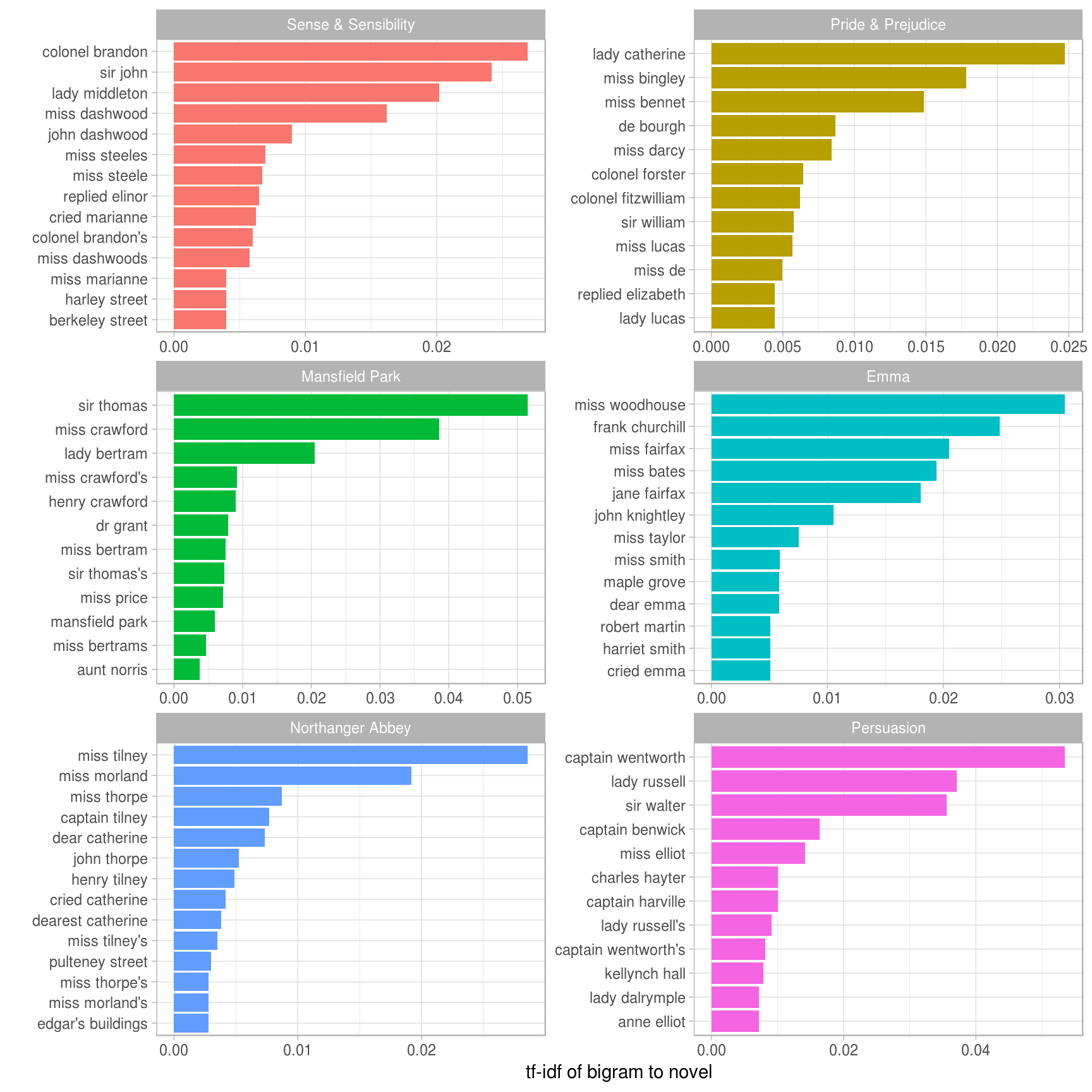
Figure 4.1: The 12 bigrams with the highest tf-idf from each Jane Austen novel
Much as we discovered in Chapter 3, the units that distinguish each Austen book are almost exclusively names. We also notice some pairings of a common verb and a name, such as “replied elizabeth” in Pride & Prejudice, or “cried emma” in Emma.
There are advantages and disadvantages to examining the tf-idf of bigrams rather than individual words. Pairs of consecutive words might capture structure that isn’t present when one is just counting single words, and may provide context that makes tokens more understandable (for example, “pulteney street”, in Northanger Abbey, is more informative than “pulteney”). However, the per-bigram counts are also sparser: a typical two-word pair is rarer than either of its component words. Thus, bigrams can be especially useful when you have a very large text dataset.
4.1.3 Using bigrams to provide context in sentiment analysis
Our sentiment analysis approch in Chapter 2 simply counted the appearance of positive or negative words, according to a reference lexicon. One of the problems with this approach is that a word’s context can matter nearly as much as its presence. For example, the words “happy” and “like” will be counted as positive, even in a sentence like “I’m not happy and I don’t like it!”
Now that we have the data organized into bigrams, it’s easy to tell how often words are preceded by a word like “not”:
bigrams_separated %>%
  filter(word1 == "not") %>%
  count(word1, word2, sort = TRUE)
## Source: local data frame [1,246 x 3]
## Groups: word1 [1]
##
## word1 word2 n
## <chr> <chr> <int>
## 1 not be 610
## 2 not to 355
## 3 not have 327
## 4 not know 252
## 5 not a 189
## 6 not think 176
## 7 not been 160
## 8 not the 147
## 9 not at 129
## 10 not in 118
## # ... with 1,236 more rowsBy performing sentiment analysis on the bigram data, we can examine how often sentiment-associated words are preceded by “not” or other negating words. We could use this to ignore or even reverse their contribution to the sentiment score.
Let’s use the AFINN lexicon for sentiment analysis, which you may recall gives a numeric sentiment score for each word, with positive or negative numbers indicating the direction of the sentiment.
AFINN <- get_sentiments("afinn")

AFINN
## # A tibble: 2,476 × 2
## word score
## <chr> <int>
## 1 abandon -2
## 2 abandoned -2
## 3 abandons -2
## 4 abducted -2
## 5 abduction -2
## 6 abductions -2
## 7 abhor -3
## 8 abhorred -3
## 9 abhorrent -3
## 10 abhors -3
## # ... with 2,466 more rowsWe can then examine the most frequent words that were preceded by “not” and were associated with a sentiment.
not_words <- bigrams_separated %>%
  filter(word1 == "not") %>%
  inner_join(AFINN, by = c(word2 = "word")) %>%
  count(word2, score, sort = TRUE) %>%
  ungroup()

not_words
## # A tibble: 245 × 3
## word2 score n
## <chr> <int> <int>
## 1 like 2 99
## 2 help 2 82
## 3 want 1 45
## 4 wish 1 39
## 5 allow 1 36
## 6 care 2 23
## 7 sorry -1 21
## 8 leave -1 18
## 9 pretend -1 18
## 10 worth 2 17
## # ... with 235 more rowsFor example, the most common sentiment-associated word to follow “not” was “like”, which would normally have a (positive) score of 2.
It’s worth asking which words contributed the most in the “wrong” direction. To compute that, we can multiply their score by the number of times they appear (so that a word with a score of +3 occurring 10 times has as much impact as a word with a sentiment score of +1 occurring 30 times). We visualize the result with a bar plot (Figure 4.2).
not_words %>%
  mutate(contribution = n * score) %>%
  arrange(desc(abs(contribution))) %>%
  head(20) %>%
  mutate(word2 = reorder(word2, contribution)) %>%
  ggplot(aes(word2, n * score, fill = n * score > 0)) +
  geom_col(show.legend = FALSE) +
  xlab("Words preceded by \"not\"") +
  ylab("Sentiment score * number of occurrences") +
  coord_flip()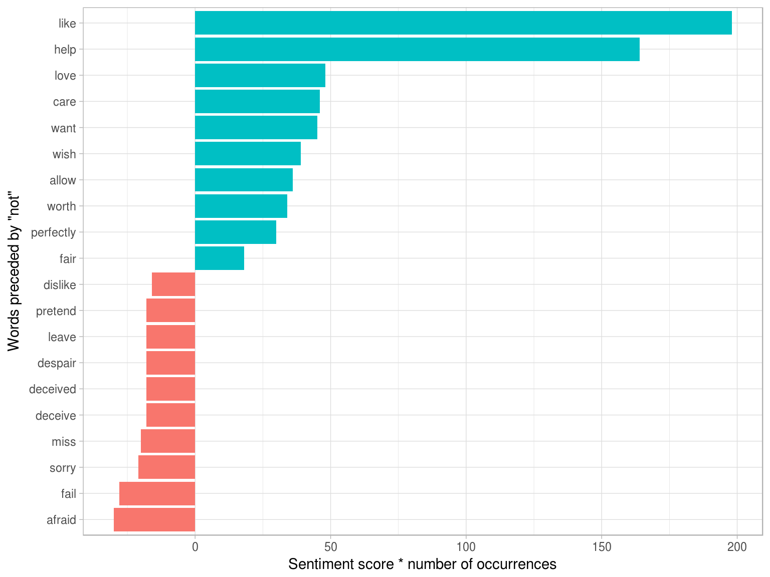
Figure 4.2: The 20 words followed by ‘not’ that had the greatest contribution to sentiment scores, in either a positive or negative direction
The bigrams “not like” and “not help” were overwhelmingly the largest causes of misidentification, making the text seem much more positive than it is. But we can see phrases like “not afraid” and “not fail” sometimes suggest text is more negative than it is.
“Not” isn’t the only term that provides some context for the following word. We could pick four common words (or more) that negate the subsequent term, and use the same joining and counting approach to examine all of them at once.
negation_words <- c("not", "no", "never", "without")

negated_words <- bigrams_separated %>%
  filter(word1 %in% negation_words) %>%
  inner_join(AFINN, by = c(word2 = "word")) %>%
  count(word1, word2, score, sort = TRUE) %>%
  ungroup()
We could then visualize what the most common words to follow each particular negation are (Figure 4.3). While “not like” and “not help” are still the two most common examples, we can also see pairings such as “no great” and “never loved.” We could combine this with the approaches in Chapter 2 to reverse the AFINN scores of each word that follows a negation. These are just a few examples of how finding consecutive words can give context to text mining methods.
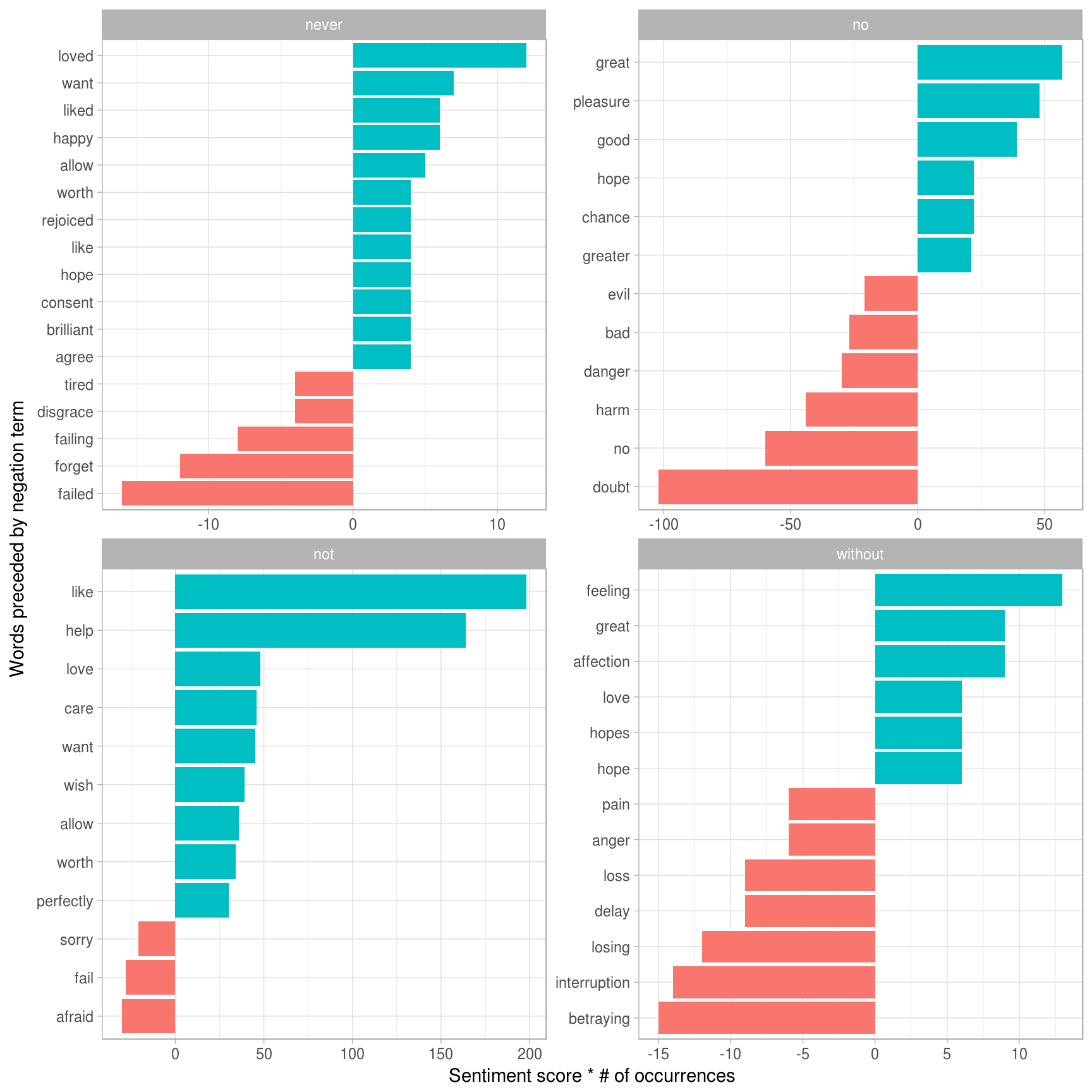
Figure 4.3: The most common positive or negative words to follow negations such as ‘never’, ‘no’, ‘not’, and ‘without’
4.1.4 Visualizing a network of bigrams with ggraph
We may be interested in visualizing all of the relationships among words simultaneously, rather than just the top few at a time. As one common visualization, we can arrange the words into a network, or “graph.” Here we’ll be referring to a “graph” not in the sense of a visualization, but as a combination of connected nodes. A graph can be constructed from a tidy object since it has three variables:
- from: the node an edge is coming from
- to: the node an edge is going towards
- weight: A numeric value associated with each edge
The igraph package has many powerful functions for manipulating and analyzing networks. One way to create an igraph object from tidy data is the graph_from_data_frame() function, which takes a data frame of edges with columns for “from”, “to”, and edge attributes (in this case n):
library(igraph)

# original counts
bigram_counts
## Source: local data frame [33,421 x 3]
## Groups: word1 [6,711]
##
## word1 word2 n
## <chr> <chr> <int>
## 1 sir thomas 287
## 2 miss crawford 215
## 3 captain wentworth 170
## 4 miss woodhouse 162
## 5 frank churchill 132
## 6 lady russell 118
## 7 lady bertram 114
## 8 sir walter 113
## 9 miss fairfax 109
## 10 colonel brandon 108
## # ... with 33,411 more rows# filter for only relatively common combinations
bigram_graph <- bigram_counts %>%
filter(n > 20) %>%
graph_from_data_frame()
bigram_graph## IGRAPH DN-- 91 77 --
## + attr: name (v/c), n (e/n)
## + edges (vertex names):
## [1] sir ->thomas miss ->crawford captain ->wentworth miss ->woodhouse
## [5] frank ->churchill lady ->russell lady ->bertram sir ->walter
## [9] miss ->fairfax colonel ->brandon miss ->bates lady ->catherine
## [13] sir ->john jane ->fairfax miss ->tilney lady ->middleton
## [17] miss ->bingley thousand->pounds miss ->dashwood miss ->bennet
## [21] john ->knightley miss ->morland captain ->benwick dear ->miss
## [25] miss ->smith miss ->crawford's henry ->crawford miss ->elliot
## [29] dr ->grant miss ->bertram sir ->thomas's ten ->minutes
## + ... omitted several edgesigraph has plotting functions built in, but they’re not what the package is designed to do, so many other packages have developed visualization methods for graph objects. We recommend the ggraph package (Pedersen 2017), because it implements these visualizations in terms of the grammar of graphics, which we are already familiar with from ggplot2.
We can convert an igraph object into a ggraph with the ggraph function, after which we add layers to it, much like layers are added in ggplot2. For example, for a basic graph we need to add three layers: nodes, edges, and text.
library(ggraph)
set.seed(2017)

ggraph(bigram_graph, layout = "fr") +
  geom_edge_link() +
  geom_node_point() +
  geom_node_text(aes(label = name), vjust = 1, hjust = 1)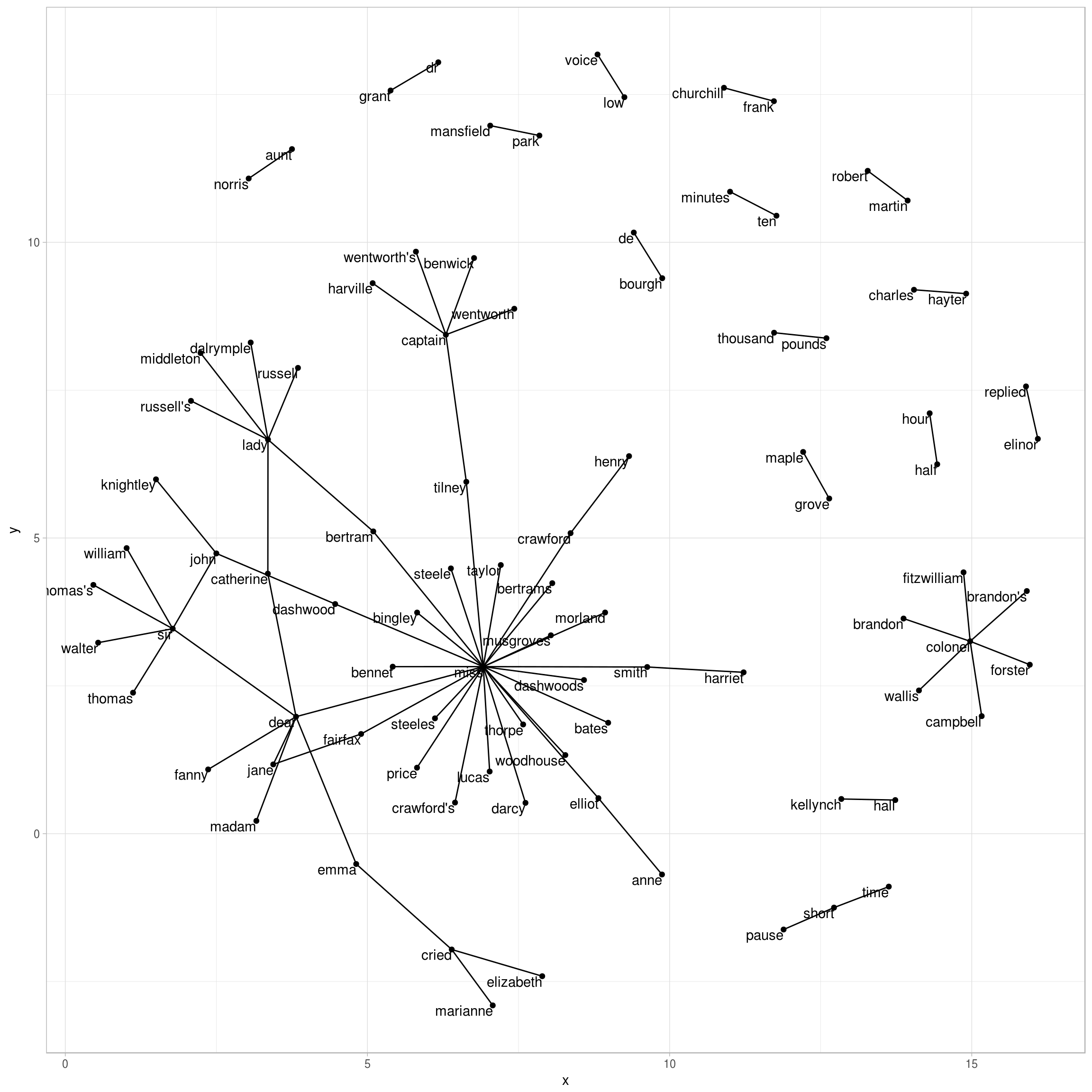
Figure 4.4: Common bigrams in Pride and Prejudice, showing those that occurred more than 20 times and where neither word was a stop-word
In Figure 4.4, we can visualize some details of the text structure. For example, we see that salutations such as “miss”, “lady”, “sir”, “and”colonel" form common centers of nodes, which are often followed by names. We also see pairs or triplets along the outside that form common short phrases (“half hour”, “thousand pounds”, or “short time/pause”).
We conclude with a few polishing operations to make a better looking graph (Figure 4.5):
- We add the
edge_alphaaesthetic to the link layer to make links transparent based on how common or rare the bigram is - We add directionality with an arrow, constructed using
grid::arrow(), including anend_capoption that tells the arrow to end before touching the node - We tinker with the options to the node layer to make the nodes more attractive (larger, blue points)
- We add a theme that’s useful for plotting networks,
theme_void()
set.seed(2016)

a <- grid::arrow(type = "closed", length = unit(.15, "inches"))

ggraph(bigram_graph, layout = "fr") +
  geom_edge_link(aes(edge_alpha = n), show.legend = FALSE,
                 arrow = a, end_cap = circle(.07, 'inches')) +
  geom_node_point(color = "lightblue", size = 5) +
  geom_node_text(aes(label = name), vjust = 1, hjust = 1) +
  theme_void()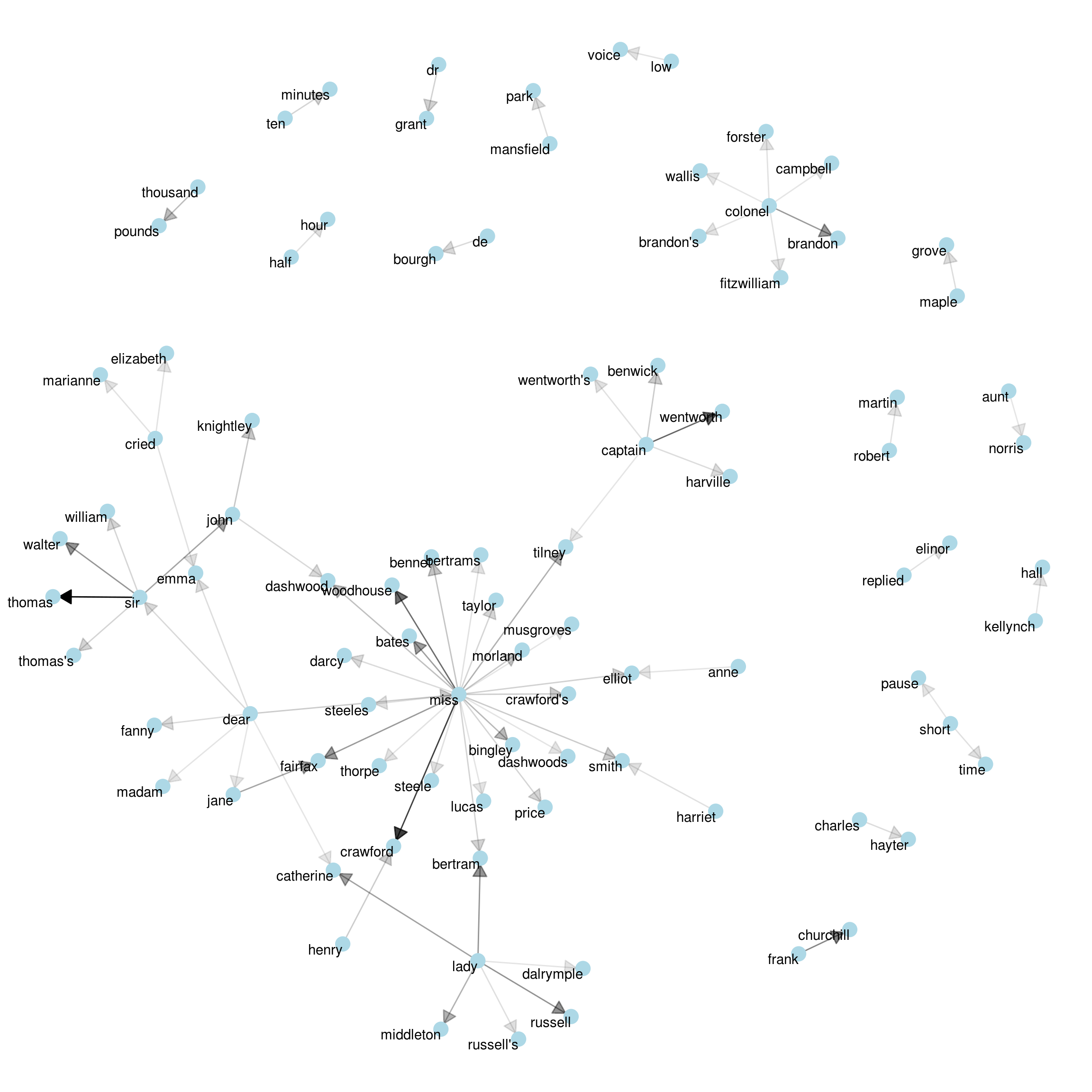
Figure 4.5: Common bigrams in Pride and Prejudice, with some polishing.
It may take a some experimentation with ggraph to get your networks into a presentable format like this, but the network structure is useful and flexible way to visualize relational tidy data.
Note that this is a visualization of a Markov chain, a common model in text processing. In a Markov chain, each choice of word depends only on the previous word. In this case, a random generator following this model might spit out “dear”, then “sir”, then “william/walter/thomas/thomas’s”, by following each word to the most common words that follow it. To make the visualization interpretable, we chose to show only the most common word to word connections, but one could imagine an enormous graph representing all connections that occur in the text.
4.1.5 Visualizing bigrams in other texts
We went to a good amount of work in cleaning and visualizing bigrams on a text dataset, so let’s collect it into a function so that we easily perform it on other text datasets.
To make it easy to use the count_bigrams() and visualize_bigrams() yourself, we’ve also reloaded the packages necessary for them.
library(dplyr)
library(tidyr)
library(tidytext)
library(ggplot2)
library(igraph)
library(ggraph)

count_bigrams <- function(dataset) {
  dataset %>%
    unnest_tokens(bigram, text, token = "ngrams", n = 2) %>%
    separate(bigram, c("word1", "word2"), sep = " ") %>%
    filter(!word1 %in% stop_words$word,
           !word2 %in% stop_words$word) %>%
    count(word1, word2, sort = TRUE)
}

visualize_bigrams <- function(bigrams) {
  set.seed(2016)
  a <- grid::arrow(type = "closed", length = unit(.15, "inches"))

  bigrams %>%
    graph_from_data_frame() %>%
    ggraph(layout = "fr") +
    geom_edge_link(aes(edge_alpha = n), show.legend = FALSE, arrow = a) +
    geom_node_point(color = "lightblue", size = 5) +
    geom_node_text(aes(label = name), vjust = 1, hjust = 1) +
    theme_void()
}
At this point, we could visualize bigrams in other works, such as the King James Version of the Bible:
# the King James version is book 10 on Project Gutenberg:
library(gutenbergr)
kjv <- gutenberg_download(10)library(stringr)
kjv_bigrams <- kjv %>%
count_bigrams()
# filter out rare combinations, as well as digits
kjv_bigrams %>%
filter(n > 40,
!str_detect(word1, "\\d"),
!str_detect(word2, "\\d")) %>%
visualize_bigrams()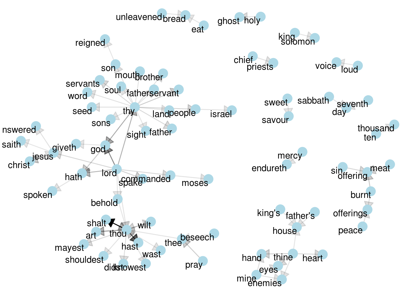
Figure 4.6: Directed graph of common bigrams in the King James Bible, showing those that occurred more than 40 times
Figure 4.6 thus lays out a common “blueprint” of language within the Bible, particularly focused around “thy” and “thou” (which could probably be considered stopwords!) You can use the gutenbergr package and these count_bigrams/visualize_bigrams functions to visualize bigrams in other classic books you’re interested in.
4.2 Counting and correlating pairs of words with the widyr package
Tokenizing by n-gram is a useful way to explore pairs of adjacent words. However, we may also be interested in words that tend to co-occur within particular documents or particular chapters, even if they don’t occur next to each other.
Tidy data is a useful structure for comparing between variables or grouping by rows, but it can be challenging to compare between rows: for example, to count the number of times that two words appear within the same document, or to see how correlated they are. Most operations for finding pairwise counts or correlations need to turn the data into a wide matrix first.
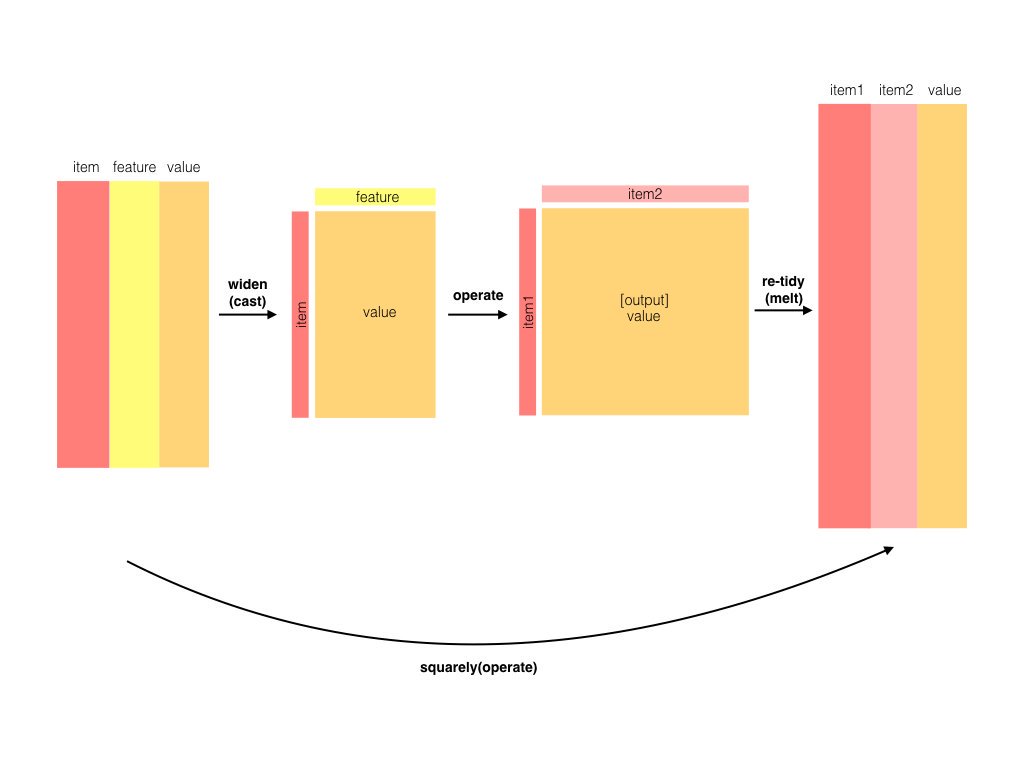
Figure 4.7: The philosophy behind the widyr package, which can perform operations such as counting and correlating on pairs of values in a tidy dataset. The widyr package first ‘casts’ a tidy dataset into a wide matrix, performs an operation such as a correlation on it, then re-tidies the result.
We’ll examine some of the ways tidy text can be turned into a wide matrix in Chapter 5, but in this case it isn’t necessary. The widyr package makes operations such as computing counts and correlations easy, by simplifying the pattern of “widen data, perform an operation, then re-tidy data” (Figure 4.7). We’ll focus on a set of functions that make pairwise comparisons between groups of observations (for example, between documents, or sections of text).
4.2.1 Counting and correlating among sections
Consider the book “Pride and Prejudice” divided into 10-line sections, as we did (with larger sections) for sentiment analysis in Chapter 2. We may be interested in what words tend to appear within the same section.
austen_section_words <- austen_books() %>%
  filter(book == "Pride & Prejudice") %>%
  mutate(section = row_number() %/% 10) %>%
  filter(section > 0) %>%
  unnest_tokens(word, text) %>%
  filter(!word %in% stop_words$word)

austen_section_words
## # A tibble: 37,240 × 3
## book section word
## <fctr> <dbl> <chr>
## 1 Pride & Prejudice 1 truth
## 2 Pride & Prejudice 1 universally
## 3 Pride & Prejudice 1 acknowledged
## 4 Pride & Prejudice 1 single
## 5 Pride & Prejudice 1 possession
## 6 Pride & Prejudice 1 fortune
## 7 Pride & Prejudice 1 wife
## 8 Pride & Prejudice 1 feelings
## 9 Pride & Prejudice 1 views
## 10 Pride & Prejudice 1 entering
## # ... with 37,230 more rowsOne useful function from widyr is the pairwise_count() function. The prefix pairwise_ means it will result in one row for each pair of words in the word variable. This lets us count common pairs of words co-appearing within the same section:
library(widyr)

# count words co-occuring within sections
word_pairs <- austen_section_words %>%
  pairwise_count(word, section, sort = TRUE)

word_pairs
## # A tibble: 796,008 × 3
## item1 item2 n
## <chr> <chr> <dbl>
## 1 darcy elizabeth 144
## 2 elizabeth darcy 144
## 3 miss elizabeth 110
## 4 elizabeth miss 110
## 5 elizabeth jane 106
## 6 jane elizabeth 106
## 7 miss darcy 92
## 8 darcy miss 92
## 9 elizabeth bingley 91
## 10 bingley elizabeth 91
## # ... with 795,998 more rowsNotice that while the input had one row for each pair of a document (a 10-line section) and a word, the output has one row for each pair of words. This is also a tidy format, but of a very different structure that we can use to answer new questions.
For example, we can see that the most common pair of words in a section is “Elizabeth” and “Darcy” (the two main characters). We can easily find the words that most often occur with Darcy:
word_pairs %>%
  filter(item1 == "darcy")
## # A tibble: 2,930 × 3
## item1 item2 n
## <chr> <chr> <dbl>
## 1 darcy elizabeth 144
## 2 darcy miss 92
## 3 darcy bingley 86
## 4 darcy jane 46
## 5 darcy bennet 45
## 6 darcy sister 45
## 7 darcy time 41
## 8 darcy lady 38
## 9 darcy friend 37
## 10 darcy wickham 37
## # ... with 2,920 more rows4.2.2 Pairwise correlation
Pairs like “Elizabeth” and “Darcy” are the most common co-occurring words, but that’s not particularly meaningful since they’re also the most common individual words. We may instead want to examine correlation among words, which indicates how often they appear together relative to how often they appear separately.
In particular, here we’ll focus on the phi coefficient, a common measure for binary correlation. The focus of the phi coefficient is how much more likely it is that either both word X and Y appear, or neither do, than that one appears without the other.
Consider the following table:
| Has word Y | No word Y | Total | ||
|---|---|---|---|---|
| Has word X | \(n_{11}\) | \(n_{10}\) | \(n_{1\cdot}\) | |
| No word X | \(n_{01}\) | \(n_{00}\) | \(n_{0\cdot}\) | |
| Total | \(n_{\cdot 1}\) | \(n_{\cdot 0}\) | n |
For example, that \(n_{11}\) represents the number of documents where both word X and word Y appear, \(n_{00}\) the number where neither appears, and \(n_{10}\) and \(n_{01}\) the cases where one appears without the other. In terms of this table, the phi coefficient is:
\[\phi=\frac{n_{11}n_{00}-n_{10}n_{01}}{\sqrt{n_{1\cdot}n_{0\cdot}n_{\cdot0}n_{\cdot1}}}\]
The phi coefficient is equivalent to the Pearson correlation, which you may have heard of elsewhere, when it is applied to binary data).
The pairwise_cor() function in widyr lets us find the phi coefficient between words based on how often they appear in the same section. Its syntax is similar to pairwise_count().
# we need to filter for at least relatively common words first
word_cors <- austen_section_words %>%
  group_by(word) %>%
  filter(n() >= 20) %>%
  pairwise_cor(word, section, sort = TRUE)

word_cors
## # A tibble: 154,842 × 3
## item1 item2 correlation
## <chr> <chr> <dbl>
## 1 bourgh de 0.9508501
## 2 de bourgh 0.9508501
## 3 pounds thousand 0.7005808
## 4 thousand pounds 0.7005808
## 5 william sir 0.6644719
## 6 sir william 0.6644719
## 7 catherine lady 0.6633048
## 8 lady catherine 0.6633048
## 9 forster colonel 0.6220950
## 10 colonel forster 0.6220950
## # ... with 154,832 more rowsThis output format is helpful for exploration. For example, we could find the words most correlated with a word like “pounds” using a filter operation.
word_cors %>%
  filter(item1 == "pounds")
## # A tibble: 393 × 3
## item1 item2 correlation
## <chr> <chr> <dbl>
## 1 pounds thousand 0.70058081
## 2 pounds ten 0.23057580
## 3 pounds fortune 0.16386264
## 4 pounds settled 0.14946049
## 5 pounds wickham's 0.14152401
## 6 pounds children 0.12900011
## 7 pounds mother's 0.11905928
## 8 pounds believed 0.09321518
## 9 pounds estate 0.08896876
## 10 pounds ready 0.08597038
## # ... with 383 more rowsThis lets us pick particular interesting words and find the other words most associated with them (Figure 4.8).
word_cors %>%
  filter(item1 %in% c("elizabeth", "pounds", "married", "pride")) %>%
  group_by(item1) %>%
  top_n(6) %>%
  ungroup() %>%
  mutate(item2 = reorder(item2, correlation)) %>%
  ggplot(aes(item2, correlation)) +
  geom_bar(stat = "identity") +
  facet_wrap(~ item1, scales = "free") +
  coord_flip()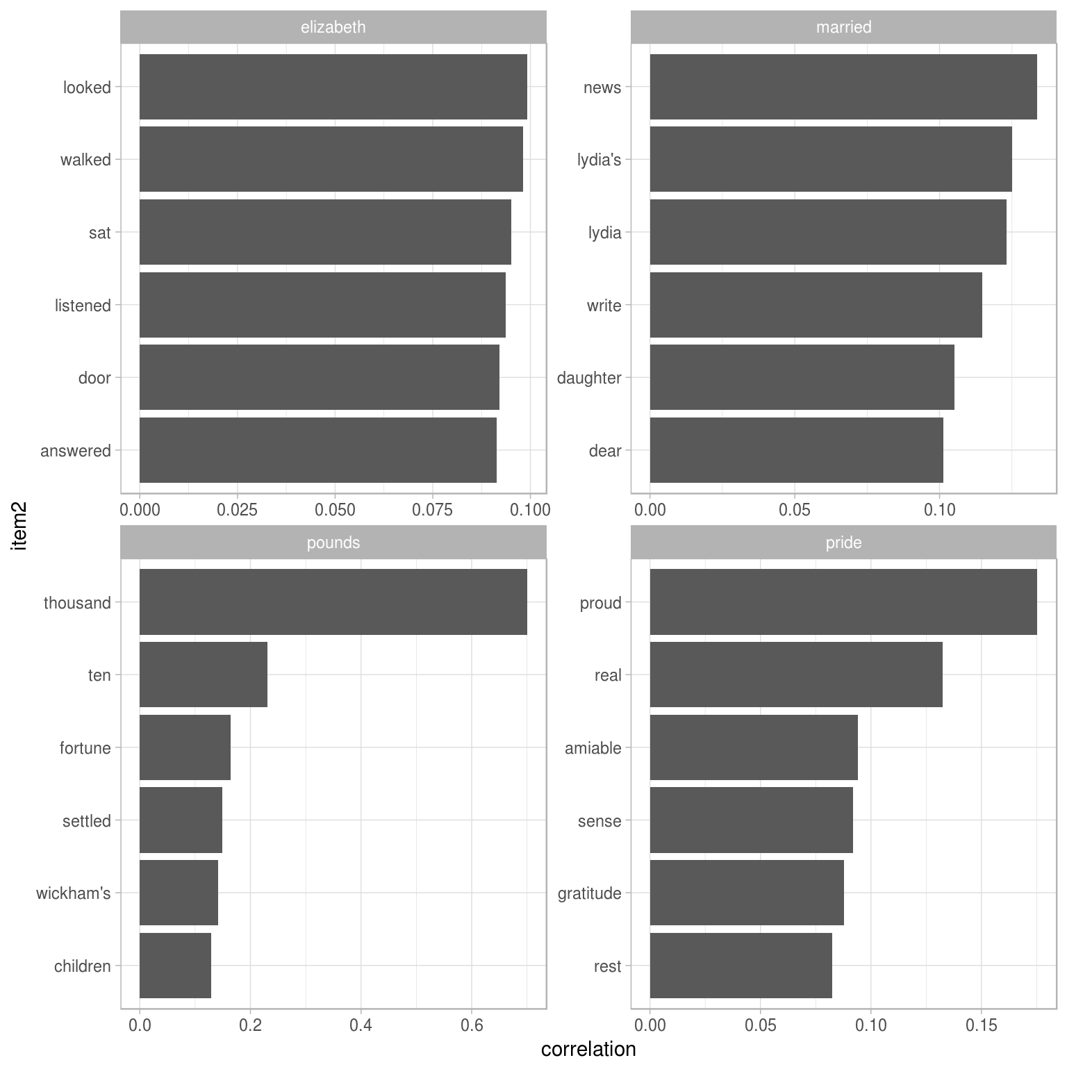
Figure 4.8: Words from Pride and Prejudice that were most correlated with ‘elizabeth’, ‘pounds’, ‘married’, and ‘pride’
Just as we used ggraph to visualize bigrams, we can use it to visualize the correlations and clusters of words that were found by the widyr package (Figure 4.9).
set.seed(2016)

word_cors %>%
  filter(correlation > .15) %>%
  graph_from_data_frame() %>%
  ggraph(layout = "fr") +
  geom_edge_link(aes(edge_alpha = correlation), show.legend = FALSE) +
  geom_node_point(color = "lightblue", size = 5) +
  geom_node_text(aes(label = name), repel = TRUE) +
  theme_void()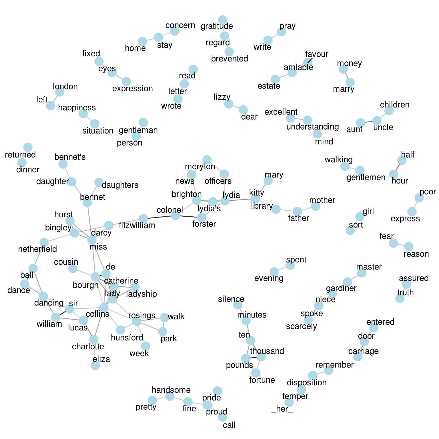
Figure 4.9: Pairs of words in Pride and Prejudice that show at least a .15 correlation of appearing within the same 10-line section
Note that unlike the bigram analysis, the relationships here are symmetrical, rather than directional (there are no arrows). We can also see that while pairings of names and titles that dominated bigram pairings are common, such as “colonel/fitzwilliam”, we can also see pairings of words that appear close to each other, such as “walk” and “park”, or “dance” and “ball”.
4.3 Summary
This chapter showed how the tidy text approach is useful not only for analyzing individual words, but also for exploring the relationships and connections between words. Such relationships can involve n-grams, which enable us to see what words tend to appear after others, or co-occurences and correlations, for words that appear in proximity to each other. This chapter also demonstrated the ggraph package for visualizing both of these types of relationships as networks. These network visualizations are a flexible tool for exploring relationships, and will play an important role in the case studies in later chapters.
References
Pedersen, Thomas Lin. 2017. ggraph: An Implementation of Grammar of Graphics for Graphs and Networks. https://cran.r-project.org/package=ggraph.